
A land manager has forty rehabilitation sites, one crew and six visits left in the quarter. The useful question for an AI system is not “Which sites have failed?” A site visit is how the manager finds that out. The useful question is which six visits are most likely to change the work plan. That distinction determines what data to buy, what compute to rent and whether a language model belongs in the process at all.
On 30 July 2025, Google DeepMind introduced AlphaEarth Foundations. The team combined observations from multiple sources, including optical imagery and radar, into a compact representation of the Earth’s surface. Google also made annual embeddings available in Earth Engine. For a small operations team, access to the computed dataset was as consequential as the model itself: it could test a field question without building a satellite-processing pipeline or training a foundation model.
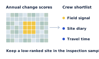
What a ten-metre cell can tell you
For each ten-metre cell, the Earth Engine dataset supplies 64 numbers that describe the cell over a calendar year. The numbers work together; the fourth value is not a vegetation meter and the tenth is not a measure of erosion. Google documents the vectors as unit length and comparable across years. Their dot product gives a measure of similarity. Subtracting that similarity from one gives a convenient change score: identical vectors score zero, and larger values indicate a greater difference in the representation.
A change score is neither a probability of damage nor an explanation. A planned earthworks programme can produce a strong signal and need no intervention. A leaking culvert in a narrow strip may matter enormously while affecting only part of one cell. An annual dataset also cannot establish that a storm last Tuesday caused a change. A team responding to this week’s storm needs recent observations. Comparing two annual summaries answers a different question.
Build a shortlist that can be proved wrong
Start with the site boundaries the crew actually uses, including which side of a fence is in scope. Compare matching cells across two annual layers; do not treat a neighbouring property as the previous state of the site. For each site, report the fraction of valid cells with a large change alongside an overall summary. A median alone can hide a disturbed corner. A maximum alone can put an entire property at the top of the list because of one boundary cell.
Choose a threshold using sites with field notes, then evaluate it on different sites. Splitting adjacent pixels from the same paddock between training and testing flatters the result: the algorithm gets to see much the same soil, weather and management history on both sides. Where site boundaries or image coverage leave too few valid cells, mark the site as unresolved. Quietly converting missing observations to “no change” builds false reassurance into the route.
Scroll to see all columns.
| Site signal | Plausible competing explanation | Action for the crew planner |
|---|---|---|
| Large, contiguous change inside the boundary | New disturbance, or the planned earthworks logged in the site diary. | Check the diary; visit if the location or extent does not match. |
| Strong change only along a fence | Adjacent land use or a shifted boundary. | Check the polygon against imagery before scheduling travel. |
| Little apparent change at a priority habitat | Stable cover, or damage too narrow for a ten-metre cell. | Retain a control visit; the score cannot clear the site. |
Measure information gained per crew day
Suppose the existing route produced two actionable findings in six visits over three crew days. A proposed route produces three in six visits but takes four crew days. On paper, the hit rate rose from 33% to 50%. Per crew day, however, the change is from 0.67 findings to 0.75, a gain of roughly 12.5%. If the remote route takes five days, it falls to 0.60. These numbers illustrate how travel can reverse a ranking; they are not field results or a prediction of model performance.
Run the comparison prospectively. Give the planner the usual route and a model-assisted alternative before the vehicle leaves. Preserve some low-ranked visits, record what each inspection found, and distinguish “maintenance required” from “change confirmed”. A perfectly detected change that was already on the work order did not create another useful finding. Six visits are too few to claim a dependable improvement. Repeat across seasons and terrain before changing an inspection schedule that protects high-consequence sites.
Put GPU hours where they can change the decision
Comparing two ready-made vectors at a few sites is a poor reason to reserve a GPU cluster. As a scale check, a square kilometre contains about 10,000 ten-metre cells. If an analyst expands 64 components to four-byte numbers in memory, one year of vectors for that area occupies about 2.56 MB before masks and overhead. Two years across forty one-square-kilometre sites would be roughly 205 MB in that representation. It is a sizing example, not the dataset’s download size. For that trial, reading tiles, aligning boundaries and getting reliable field labels may dominate the work.
The computation changes if the team needs fresh high-resolution imagery and trains a segmentation model against labelled damage. Now there are image chips to decode, augment and move into accelerator memory; training runs to repeat; and a model to score against held-out sites. Time a representative slice end to end. If the GPU waits for storage, renting more GPUs can increase the bill without getting the map to the crew any earlier. A useful infrastructure brief gives the image dimensions, batch size, precision, measured data throughput and the deadline for a usable map.
Give the language model the work order, not the pixels
A model API has a narrower role. Once the geospatial pipeline has produced a shortlist, an application can send approved site IDs, survey dates, reasons for selection and known caveats to a language model for a draft crew brief. The map calculation should remain reproducible without that model. Test the draft for invented causes, swapped site IDs and phrases such as “vegetation loss confirmed” where the input said only “change detected”. Evaluate it against the time a planner takes to correct and issue the brief.
If procuring model access through Cooma Model API, size that text workload by briefs, input length, review cost and the permitted data boundary. The raw imagery need not travel with a set of site identifiers. The result is an unusually clear buying decision: pay for existing embeddings while they answer the field question, rent accelerators when a measured image workload warrants them, and spend tokens when they reduce the time between an analyst’s shortlist and a useful day on the ground.